Author: Farkas, Jeremy M.

Matt Orsagh, CFA, CIPM
Senior Director, Capital Markets Policy, Americas, CFA Institute

Climate change is arguably the biggest problem ever
faced by humanity. The good news is that we know what
the solutions are. The bad news is that the solutions will
require most people on earth to change how they live.

The physics behind climate change are simple. There
has always been some carbon dioxide (CO2) in our atmosphere.
Throughout most of human history, that level
has been in the range of 200 to 300 parts per million
(ppm). That number sounds incredibly low, but because
greenhouse gases trap heat and keep it from escaping
back into space, relatively small increases can have
a profound impact. Think of greenhouse gases in the
atmosphere as a blanket warming the earth. The higher
the concentration of greenhouse gases, the thicker that
blanket becomes. In 2021, the atmosphere’s average
ppm is about 415, and it is rising at a rate of about 1
ppm to 2 ppm per year.

Physical Risks Are Largely Baked In, But Transition Risks Are Up to Us

Greenhouse gases (GHGs) trap heat in the atmosphere.
The more GHGs we put into the atmosphere, the more
heat they trap. This cycle raises the atmosphere’s temperature,
contributing to several follow-on problems.

A hotter planet means more drought, more famine, more
extreme weather events, more property damage, and
more dislocation of humanity than any of us have seen.
We cannot know on what calendar date these disasters
will arrive, but we can be confident that they will. The
business community needs to incorporate these new
realities into our analysis to help efficiently allocate
capital in a world where the effects of climate change
are increasing. Climate change will affect every company
and every investor on earth.

Businesses need access to material data on climate
change to make the most informed investment decisions
possible. We need a robust market price on carbon
emissions; we need timely, comparable, and audited
data on material climate-related metrics; and we need
to know how the companies we invest in are responding
to climate change.

Estimates of the costs of climate change vary widely,
but all contain bad news. If no action is taken to limit
climate change, losses could be between $4 trillion and
$20 trillion), according to a 2019 estimate by Sarah Breeden,
then the Bank of England’s executive director
of international banks supervision.¹ The cost of adapting
to climate change in developing countries could
rise to between $280 billion to $500 billion per year by
2050, according to a recent United Nations Environment
Programme report. Climate change could slash up to
one-tenth of U.S. gross domestic product annually by
2100, according to the Fourth National Climate Assessment,
published in 2018 by the U.S. Global Climate
Change Research Program. That figure is more than
double the losses of the Great Recession of 2008–2009.

Physical Risks/Transition Risks and Opportunities

A hotter world will increase heat stresses and coastal
flooding due to more storm surges and rising sea levels
from ice melting in the Arctic and Antarctic. This is
already increasing the cost of insuring coastal areas
as insurance companies change their rates every year,
with dire implications for some coastal properties and
homes with long-term financing.

Hotter oceans give hurricanes more power, and hotter
air holds more moisture, creating stronger and more
damaging hurricanes and thunderstorms.

The earth’s oceans are actually larger carbon sinks—
things that absorb more carbon than they release— than
the trees and plant life that we usually think of as the
main check against carbon dioxide in the atmosphere.
This, however, leads to a warming ocean with higher
acidity levels, which is a problem because about 40%
of the world’s population lives within 100 kilometers
of the coast, and 4.3 billion people rely on fish for 15%
of their animal protein.² Investors need to understandfesti
the impact of climate change on our oceans to grasp its
impact on businesses that depend on the sea and what
comes from it for their livelihoods.

Terrestrial food sources will also be challenged, as—if
there is no change in current growing regions—weighted
average yields are predicted to decrease by 30%–46%
before the end of the century.³

These physical risks are well known because we see them
in the headlines. But just as important are the transition
risks that a reaction to climate change will bring. In the
coming years and decades, whole industries will be
transformed. Oil and gas, utilities, and transportation
are the sectors that will be most affected, but no industry
will be untouched by climate change.

As businesses, regulators, and policymakers react to
climate change by moving to a low-carbon economy in
the coming decades, that transition will have profound
effects on businesses. It is important that businesses
understand the changes coming, their relative timing,
and the likely impact on their businesses, so they can
plan for it. Businesses that fail to do so will be left at
a severe disadvantage compared with companies that
manage the transition well.

What Can Businesses Do?

Climate change isn’t “coming.” It is already here. “Hundred-
year floods” are coming every 10 years, making
flood maps based on historical weather patterns all
but obsolete. Extreme heat is making droughts more
extreme and longer-lasting, already stressing water
resources in the western U.S. and increasing the number
and severity of forest fires. But business and finance can
only do so much. The real big lifting on climate change
will take changes in behavior, which requires changes
in incentives. Governments can set these incentives, so
business and finance should work with policymakers
to iron out what to do.

3 Recommendations for Action

1. Set a price on carbon—Adopting a price on carbon
is essential for combating climate change, which must
be supported by a transparent pricing mechanism that
enables businesses to reliably incorporate carbon pricing
into their analysis of investments’ exposure to climate
risk. CO2 and other greenhouse gases in the atmosphere
are negative externalities—effects that aren’t priced
into the cost of goods and services—that are not yet
widely priced.
About 20% of global emissions are priced by some sort
of carbon market. Europe, China, New Zealand, and
others, including the east and west coasts of the U.S.
operate under some kind of carbon pricing mechanism.
But the reach of carbon markets needs to expand to
eventually provide consumers and businesses with the
incentive to move away from carbon. CO2 and other
greenhouse gases are a negative externality that needs
to be priced to adequately address the negative effects
of climate change.

It is important that policymakers ensure that regulatory
frameworks for carbon markets are designed to deliver
transparency, liquidity, ease of access for global market
participants, and similar standards across jurisdictions,
to underpin robust and reliable carbon pricing.

2. Include carbon price expectations in business
strategy—A realistic market price on carbon will send
a price signal that businesses and consumers need to
properly value the externalities that come with greenhouse
gas emissions. The externality of climate change
has a cost, and that cost will be the future impact of
climate change on our markets and society. Economists,
investors, and policymakers who have studied the issue
agree that a realistic price on carbon will allow markets
to do the heaviest lifting in combating climate change.

3. Increase transparency and disclosure on climate
metrics—Businesses should work with investors, policymakers,
and stakeholders to settle on the metrics that
matter when assessing a company’s climate-change
strategy. Investors, policymakers, and stakeholders
often lack the data needed to make informed decisions
on climate investment and policy. Businesses should
work with these groups to determine what information
(scope 1,2, and 3 emissions, for example) is needed to
make the best policy and investment decisions around
the issue of climate change.

Conclusion: Risks and Opportunities

The bad news is that climate change is one of the largest
economic and societal challenges that mankind has ever
faced. The good news is that we know the solutions to the
problem. However, this will require changes to how we
live, including the way we eat, farm, travel, do business,
and invest. Addressing and adapting to climate change
will be a cultural change for all of us, from the individual
to the largest corporation. But those changes contain
as much opportunity as they do risk. Those who can
adapt best to the changing landscape and seize those
opportunities will find the most benefit.

References

¹ 2015 report from the Economist Intelligence Unit.

² Global Environment Facility, “Fisheries.”

³ Wolfram Schlenker and Michael J. Roberts, “Nonlinear Temperature
Effects Indicate Severe Damages to U.S. Crop Yields under Climate
Change,” Proceedings of the National Academy of Sciences (15 September
2009).

Dear Friends and Colleagues,

The past year has been challenging to say the least and we have experienced things during the last year that are unprecedented. On behalf of myself and the rest of the board members of CFA Society Baltimore, I hope your families are safe and well during these times.

The CFA Society Baltimore was not immune from the affects of the COVID-19 pandemic and we had to change our business model on the fly, as many other businesses were forced to do the same. We shifted our focus from our traditional programming events at the Center Club, to virtual events and explored different types of content to connect and engage our membership.

Despite all the change in the past year, we still have been able to produce this year’s Baltimore Business Review. This is the twelfth edition of the Baltimore Business Review and we are extremely proud of this publication. This year’s Baltimore Business Review represents an ongoing partnership between the business and academic communities in Baltimore. CFA Society Baltimore is incredibly fortunate to have a great partnership with the Towson College of Business and Economics to make this world-class publication possible, despite everything going in the world right now.

This publication would not be possible with the help and support of our publication team. I want to thank the editor staff of Susan Weiner, and Lijing Du and Rachel Gordon from Towson University. I want to also thank the many contributors to this year’s edition and to Rick Pallansch and Chris Komisar from the Towson University Creative Services team. Your time and efforts are incredibly valuable.

The CFA Society Baltimore originated in 1948 and currently serves over 750 members today. In a joint effort, the CFA Society Baltimore and its parent company, the CFA Institute, work to promote and advocate the principles of the CFA program. The society proudly leads the investment community and other finance related communities by promoting the highest standard of ethics, education, and professional excellence for the benefits of the entire community. In this publication, you can see the list of the top ten employers of our society’s members.

During the past year, the CFA Society Baltimore has worked with Baltimore leaders to expand our efforts in diversity and inclusion in the investment management profession. We have, and will continue to listen to business and community leaders to learn the challenges of diversity and inclusion in the investment management industry in Baltimore. The leaders of the CFA Society Baltimore recognize that we are in a unique position in that we are a conduit between the investment management profession, academic institutions, and community organizations. We have set forth a plan and have put our time, effort and resources in making sure our goals and objectives are met with respect to diversity and inclusion.

I hope you enjoy this publication and find its content engaging and enriching. As always, we welcome your feedback and insights. To learn more about how CFA Society Baltimore can help support your career and professional network, please visit our website or find us on social media.

Zachary C. Reichenbach, CFA, CPA/ABV/CFF
President, CFA Society Baltimore

Dear Colleagues and Friends,

I take great pleasure in sharing with you the twelfth issue of the Baltimore Business Review: A Maryland Journal. Year after year, Baltimore Business Review leverages the relative strengths of the College of Business and Economics (CBE) at Towson University and the CFA Society Baltimore to create an outstanding resource which showcases opportunities in the Baltimore and Maryland business communities and beyond.

Consistent with our vision, this issue covers a variety of topics from a diverse range of voices and perspectives, including scholars, local business practitioners and students. In this issue, we showcase how a Maryland family business continued to emphasize their values throughout the pandemic, highlighting what they have learned, and what other local businesses can take away from their experience. We discuss current trends in live music and the impact of the pandemic on the industry. You will also find an article collaboratively produced by a student and faculty member addressing the use of data analytics in the pharmaceutical industry. Further, we focus our attention on the market reaction to the announcement of tariffs on Chinese goods, as well as present a study from the Towson University Investment Group on students’ knowledge of retirement and financial planning concepts.

I would like to express my appreciation to our editors and contributors to this issue of the Baltimore Business Review. It is their generous contributions of time and effort that made this publication possible. We are delighted that you are joining us as readers, and as always, we look forward to hearing any feedback.

Best regards,

Shohreh A. Kaynama, Ph.D.
Dean, College of Business and Economics

Sarah Pulkowski
President, Towson University Investment Group

Jacob Piazza
Portfolio Manager, Towson University Investment Group

Keyur Patel
Vice-President, Towson University Investment Group

Aleksandr Olshanskiy
Compliance Officer, Towson University Investment Group

Introduction

The Towson University Investment Group (TUIG) conducted
a survey concerning the extent to which Towson
University students have knowledge of retirement and
financial planning concepts. Basic demographic and education-
related information was first queried, followed
by retirement planning and respondents’ knowledge
of available financial instruments. In total, we had
26 respondents. With the existing macroeconomic
backdrop as it currently stands – divergence between
the S&P 500 and SMID cap equities, and treasuries
at an all-time low after accommodative actions by the
Fed – retirement planning, we surmised, is especially
important for new college graduates. Key questions
in the survey included: When do you want to retire?
How much do you need to retire? What percent of
your income do you save for retirement each year?
How much money do you expect to live on each year
while in retirement?

Towson University is composed of the following colleges:
College of Business & Economics (CBE), College
of Health Professions (CHP), Jess & Mildred Fisher
College of Science & Mathematics (FCSM), College
of Liberal Arts (CLA), College of Fine Arts & Communication
(COFAC), and College of Education (CE).
The students questioned were segmented by college.
Allowing for inter-college and intra-college comparisons.
In addition to segmenting students by college,
we also segmented students by major. We conducted
the survey in October 2020. With the results of the
survey, we were able to show how Towson University
students are preparing for retirement, and their overall
knowledge of retirement.

Participant Background

The demographics data from our respondents indicates
no particular skew to any given population; 53.6% of
our participants are between 20-21, while 53.6% are
male. In terms of ethnic distribution, respondents were
28.6% Black/African American and 32.1% Caucasian,
with the remainder being distributed between Hispanic,
Asian, and Native American ethnic groups. We saw a
moderate skew towards older students, with more than
80% of respondents having more than 60 credits (Junior
and Seniors), which we believe is more applicable to our
initial goal of evaluating college graduates’ knowledge
of retirement planning concepts.

In seeking to evaluate the sources of retirement planning
knowledge, and the potential impact of education
by parents, we asked respondents the extent of their
parents/ education. More than 80% of respondents’
parents have earned undergraduate degrees or gone on
to complete post-graduate education, while only 15%
of respondents’ parents had high school diplomas. As
graduates of higher education make, on average, more
income than those having only graduated high school,
we concluded that respondents had a clear skew towards
belonging to middle to higher income households. As
for respondents’ employment, more than 70% were
employed or interning in some capacity. Of the 70%
employed, the majority were employed for wages, either
salaried or paid by the hour.

While students from every college were among the
respondents (save Education), there was a preponderance
of students from the College of Business &
Economics (CBE). Over 15 students from CBE answered
our survey, the majority of which are majoring in
Finance or Financial Planning. The average GPA for
respondents was 3.25, with a range between 2.1 and 4.0.

Retirement Planning

Of our samples, 21.4% of respondents stated they
plan to retire at the age of 65. The average and median
planned retirement age, 55 and 60 years old, respectively,
indicated that, on average, students planned to
retire five years or more before the full retirement age.
Despite the full retirement age for individuals born
after 1960 increasing to 67, TU students plan to retire,
on average, at 55 years of age. TU students’ average
planned retirement age is also 7 years before they are
entitled to begin receiving social security payouts. At
age 62, the earliest that an individual can receive social
security benefits, only 70% of the social security benefits
are received. By retiring early, the accumulation period
is reduced while the distribution period is increased,
creating the real risk that a retiree will outlive their
retirement savings. Table 1 presents a comparison
between the ideal scenario for retirement planning and
the situation based on our survey.

We report the summary statistics of key survey questions
in Table 2. The median and average savings respondents
indicated as being sufficient for retirement were
$1,000,000 and $13,300,000, respectively. As far as
yearly cash flow needed in retirement, on average
respondents stated that they would need $125,000 in
retirement. These numbers conclude that students need
to make sure they create or have a long-term retirement
plan created that is updated and monitored for them
to achieve retirement success.

Towson University’s Financial Planning coursework
teaches basic calculations required for retirement planning.
If a person states to save early in life for retirement,
with an appropriate savings rate, they can accumulate
enough savings for a comfortable retirement. The ideal
scenario’s saving rate for a person in their early twenties
is 11%-13%.

With answers varying from $500,000 to $20,000,000,
students have a wide range of expectations for savings
required to retire. The majority of the respondents said
they will save $1,000,000 in preparation for retirement.
With the assumption of 2% inflation and 8% annual
return on the investment, this gives inflation adjusted
return of 5.88% during their retirement. Based on
the previous assumptions, if they save $1,000,000
by the time they retire, individuals will have $73,057
of annual distributions from their portfolio during
retirement. The present value of the expected annual
spending is $33,749. This return is based on aggressive
investing even during retirement. These calculations
should be reviewed with consideration that a modest
change in inflation, retirement life or return on the
portfolio will have dramatic effect on the disposable
income of a retiree.

Additionally, 10.7% of students have not saved anything
for retirement. Since reviewing the survey results and
expectations of retirement income, we see that most
students are not seriously preparing for retirement.
Standard guidelines of financial planning state that,
in order to retire, one must save at least 10% of their
annual income.

In addition to consistently saving income, retirement
account strategies should be considered while planning
for retirement. We surveyed students on their expectations
regarding tax rates and their knowledge on the
relation between tax and social security. Overall, students
predict an increase in taxes due to inflation and
the overall long-term impacts of Covid-19. Students
at Towson University have a broad understanding
of how this government funded retirement program
works, perceiving it to be the following¹: “Social Security
is government provided disability and retirement
income. For most citizens, after the age of 75, one can
receive social security. Before then, social security taxes
6.2% are taken out of each paycheck for employed
individuals. It is a form of compensation for older
citizens, citizens with disabilities, and citizens that
are widow(er)s.” Social security benefits, in actuality,
can be received as early as 62 (with penalties), and by
67 without penalties. Each individual’s social security
benefits vary depending on how much they earned and
how long they contributed to social security. 14 out of
26 respondents (53.9%) were able to correctly answer
basic questions regarding Social Security, while the
remaining had no knowledge or with misconception.

Though many students do not have a complete knowledge
of retirement, nor have they adequately planned
for retirement, 76% of students indicated that they will
seek financial planning advice in the future. Seeking the
advice of a Financial Professional will help to ensure that
one will be able to enjoy their golden years and possibly
extend the number of golden years an individual may
enjoy. The answers provided by students demonstrate
that those who are studying finance related subjects
have an excellent understanding of Social Security,
Retirement Planning, and Alternative Investments. The
survey conducted by the Towson University Investment
Group finds that Towson University is producing individuals
who are capable, well educated, and aware of
the current economic and financial market conditions.
Towson University is producing individuals who can
network and rely on each other to meet the demands
of knowledge that all aspects of life require, including
financial planning and retiring.

¹Definition was created by compiling the correct or partially correct
answers from respondents.

Michaël Dewally
Associate Professor, Department of Finance, Towson University

Yingying Shao
Associate Professor, Department of Finance, Towson University

On March 22, 2018, “President Trump put China
squarely in his cross hairs” according to The New York
Times. The White House had just announced tariffs on
$60 billion worth of Chinese goods. The announcement
was part of continued economic tension between the
two nations. The current White House administration
had shifted its stance on economic relations with
China. Rather than encourage trade with China and
rely on China’s efforts to participate in rules-based
agreements, the administration sees its trading partner
as an economic adversary. The decision is a reaction to
questions of fairness of trade with its partner, the U.S.
accusing China of trying to obtain American technology
and trade secrets.

The timing, magnitude and coverage of the tariffs were
unprecedented. This action came at a time when production
sharing across the two countries is at an all-time
high. The market reaction to this escalating trade war
was immediate. We document the varied reactions as
we report the stock price movements for all firms in the
U.S., firms in the Maryland-Delaware-Pennsylvania-
Virginia region and across industries.

The administration had two weeks to reveal the list
of targeted products. The market reaction on these
early days was knee-jerk as the White House had not
sketched out full details of the products that would be
subject to the 25% tariff. The market reacted strongly
negatively. The tension had been building with trade
partners but the White House actions had not targeted
a single trade partner as much up to this point. The
steel and aluminium tariffs announced earlier in March
2018 hit China to a much smaller extent, most of those
tariffs impacting Canada. This new announcement
had the potential to hurt companies for two reasons.
First, firms with suppliers in China would see their
input costs increase as tariffs would raise the prices
of Chinese goods, and would increase the demand for
and the prices of alternate suppliers’ goods. This would
guarantee profit margin pressures for these companies,
if not outright disruption. Second, firms that sell to
China would likely suffer as China was to inevitably
retaliate. The Chinese reaction was in fact immediate
with its own tariffs announcement the following day.

Following the steps of Huang et al. (2020), we focus
our study on the market reaction over the three trading
days surrounding the announcement. We report not
only the 3-day cumulative raw returns (CRR) but also
the market-adjusted cumulative abnormal returns over
the same 3-day window (CAR).

How do stocks of firms in the Maryland-Delaware-Pennsylvania-Virginia region react?

Using data from The Center for Research in Security
Prices, we collect information on all actively traded
firms that are headquartered in Maryland, and the three
states surrounding Maryland. We retrieve information
on 199 firms and proceed to compute the CRRs and
CARs for our sample. We report the results in Table 1.

Table 1 provides summary statistics for CRR and CAR for
the entire U.S. sample of listed firms, excluding financial
firms, as reported in Huang et al. (2020), and the statistics
for the regional sample we created. Overall, the market
reaction to the announcement pushed returns down a
nearly full 3%. The CARs match that number as well.
The distribution is fairly symmetric as Mean and Median
are close to each other. For our regional sample, the raw
reaction is similar to that of the entire nation, showing
a swift negative reaction to the announcement. The
CARs evidence though shows a more muted regional
reaction than nationwide. This evidence requires further
investigation. On the one hand, it hints at a lower reliance
on China for imports and exports. On the other
hand, it highlights smaller headways in trade with the
U.S. largest single-country trading partner. Regardless
of the outlook on the situation, the region’s response
to the announcement was muted.

Observations from the disruption of supply chain from
and potential impairment of sales to China suggest
that firms involved in Manufacturing sectors would
suffer a stronger response to the trade war announcement
than firms in Non-Manufacturing sectors. We
next investigate the causes of the market reaction in
relation to industry distributions. Table 2 splits the
regional sample into two sub-samples. It is clear from
this table that Manufacturing firms suffer the most
from the announcement. Manufacturing firms in the
region experienced an average loss of 3.8% whereas
Non-Manufacturing firms lost only 2.6%. In abnormal
returns term, the Non-Manufacturing sector showed no
reaction (0.0% on average) while the Manufacturing
sector lost 0.8%.

How do stocks of firms in Maryland react?

Were Maryland firms affected differently than their
counterparts in the region? Table 3 reports similar
statistics to the previous tables. In Table 3, we focus
entirely on Manufacturing firms, those firms most affected.
We separate the Maryland group from those
for the entire region. Maryland Manufacturing firms
in general experienced a smaller stock market decline
than firms in the region. The average CAR for Maryland
firms was only -0.2% compared to -0.8% for the region.

Variations nationwide and within the region are certainly
attributable to the distribution of sector activities in
each state. In order to control for these variations in
aggregate, we use Huang et al. (2020)’s methodology
and introduce an industry level measure of Chinese
Import Penetration (IP). Defined as the ratio of Chinese
Imports in the industry to the sum of the industry’s
Shipment Value plus Imports minus its Exports, the
IP measure captures the industry’s “direct trade exposure”
by measuring “the perceived reduction in import
competition from and exports to China.” Huang et
al. (2020) find a positive relationship between IP and
CAR: firms in an industry where Chinese imports are
prevalent will benefit from the enactment of tariffs as
the reduced competition from Chinese products will
boost domestic companies’ profits.

We compute the IP for firms in our sample at the 3-digit
SIC level¹. For example, SIC Code 211 for the Cigarettes
industry has a low IP of -0.19 as the industry faces little
competition from Chinese imports. Meanwhile, the IP
of SIC Code 282 for Plastic Materials is a high 0.43
as the industry faces severe competition from Chinese
imports. On balance, given the values in Table 3, we
would expect the aggregate IP of Maryland firms to be
higher than the region’s aggregate IP as the MD CARs
are higher than the region’s. Our computation shows
an IP for the MD firms of 0.09 while the IP for firms in
the other 3 states is 0.12. A further look at the distribution
of Manufacturing in Maryland versus the region
shows that only 3 out of 17 (18%) MD firms have an
IP over 0.1, while, in the rest of the region, 34% (13
out of 38) have an IP in excess of 0.1. That is, firms in
the region are in industries that face more competitive
pressures from Chinese imports. These findings are the
opposite of those from the general regression results
in Huang et al. (2020). This shows that using industry
aggregated levels of exposure to Chinese competition,
while helpful on a large scale, can hide variations within
the industry itself.

Given the limitations of the IP measure exposed above,
we turn to individual stock’s reactions on the day of
the announcement. In particular, we focus on those
firms’ recorded exposure to the Chinese markets. In
Maryland, we contrast the market reactions of U.S.
Silica and W.R. Grace. On the one hand, U.S. Silica had
a +2.2% raw return over the 3-day period. U.S. Silica
does not report any international sales nor international
suppliers in its most recent annual report. The nature
of U.S. Silica’s business leaves the company insulated
from any direct impact from the trade war. On the other
hand, W.R. Grace’s stock price dropped 6.2% over the
same time period. W.R. Grace’s exposure to China is
manyfold. W.R. Grace maintains both production and
credit facilities in China. W.R. Grace’s revenues from
Asia-Pacific represents nearly 25% of its $1.93 billions
in sales for 2018. As such, W.R. Grace was primed to
suffer from the trade war. Universal Security Instruments
is similarly exposed to Chinese imports as it has a joint
venture in Hong Kong supplying it with components.
Universal Security Instruments’s stock price dropped
3.2% on announcement. In the region, United States
Steel in PA experienced the steepest drop of 12%. The
surprise announcement of the new tariffs reiterated the
administration’s resolve in its new trade policies and
dealt a new blow to the steel manufacturer.

More than the direct adverse impact to companies’ stock
prices, the trade war imposed a concern for the State of
Maryland. According to Trade Partnership Worldwide’s
white paper on the projected impact on the U.S. economy
of the trade war, over 800,000 jobs in Maryland are
supported by trade. Of these, 18,800 are threatened
by the trade war. The enacted tariffs impacted 3% of
the Port of Baltimore’s annual tonnage. In December
2018, a survey by the Maryland Chamber of Commerce
revealed that 54% of its members reported that current
trade policies negatively affected their businesses. While
the COVID-19 pandemic has slowed down trade talks
with China, unresolved issues around trade remain a
threat to Maryland businesses.

Reference

¹Data source: https://sompks4.github.io/sub_data.html

Landler, Mark and Tankersley, Jim, Trump Hits China with Stiff
Trade Measures (March 22, 2018), The New York Times.

Huang, Yi and Lin, Chen and Liu, Sibo and Tang, Heiwai, Trade
Networks and Firm Value: Evidence from the US-China Trade
War (April 30, 2020). Available at SSRN: https://ssrn.com/
abstract=3227972 or http://dx.doi.org/10.2139/ssrn.3227972

Maryland Chamber of Commerce – https://mdchamber.org/maryland-
chamber-talks-tariffs/

Trade Partnership Worldwide, LLC, Estimated Impacts of Tariffs
on the U.S. Economy and Workers (February 2019), https://
tradepartnership.com/wp-content/uploads/2019/02/All-Tariffs-
Study-FINAL.pdf

Bradford Muir
Supervisor at Vallit Advisors

The COVID-19 pandemic has uniquely challenged
businesses; no business model or industry appears
to be immune. However, situations vary. Some
companies have been forced to adapt to avoid shuttering,
while others are riding out state-mandated
closures using cash on hand and Paycheck Protection
Program (PPP) loans. As a result, the effects of
COVID-19 on business valuations of privately held
companies can vary dramatically.

The pandemic has notably affected business valuations
through the discount rate used in the income approach
to valuation, in which projected future cash flows are
discounted to present value using a discount rate. This
article discusses the significance for valuations of privately
held businesses of (1) volatility and risk, (2) the
build-up method for determining the discount rate, and
(3) the effects of the COVID-19 pandemic on risk and
the equity discount rate for privately held businesses.

Volatility and Risk in the Global Pandemic

Volatility and risk matter because they affect what
buyers will pay for privately held businesses. Since the
pandemic’s start, U.S. equity markets have experienced
significant changes in volatility that are at least partly
tied to people’s perception of risk in those markets.
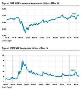
U.S. equities, as measured by the S&P 500 index, fell
more than 33% in the one-month period from February
20 to March 20 (Figure 1). However, they have
recouped these losses, eclipsing their late-February
high in late August.¹

In addition, equity market volatility, which acts as a
gauge of investor sentiment, has hit levels of volatility
unknown since the 2007–2008 financial crisis. As shown
in Figure 2, the CBOE Volatility Index (VIX) soared
from 15.6 on February 20 to a record high of 82.7
less than 30 days later on March 16, due to the rapid,
unchecked spread of the coronavirus. Values greater
than 30 for the VIX, which represents the implied volatility
of 30-day options on the S&P 500, are generally
associated with a large amount of volatility because
of investor fear or uncertainty, while values below 20
generally correspond to less stressful, even complacent,
market conditions.

Despite efforts by the Federal Reserve and Congress to
stabilize equity markets, the VIX remained significantly
above pre-pandemic levels throughout the summer.
Volatility has remained high over the 60-day period
ended November 19 as the United States and many
European nations have seen a resurgence in new coronavirus
cases.

Risk is associated with volatility. The tighter the probability
distribution of returns for an investment in
the existing economic conditions, the lower the risk
profile of the investment. In other words, risk can be
defined as, “the degree of uncertainty (or lack thereof)
of achieving future expectations at the times and in
the amounts expected.”²

In business valuation, risk is evaluated, quantified, and
accounted for in the discount rate. A discount rate is a
rate of return used to convert a monetary sum, payable
or receivable in the future, into its present value.³ The discount
rate is equal to the “cost of capital,” the expected
rate of return that the market requires to attract funds
to a particular investment.⁴ Thus, the cost of capital
is based on the principle of substitution, in that it is
equal to the return that could be earned on alternative
investments with a similar level of risk.

Other terms used interchangeably to describe the cost
of capital include:

• Rate of return
• Required rate of return
• Cost of equity capital
• Weighted average cost of capital
• Alternative cost of capital
• Discount rate
• Hurdle rate

Risk and return are positively correlated. The greater the
perceived risk of an investment, the higher the required
rate of return an investor would demand from the
purchase of the investment. Accordingly, the discount
rate and value are negatively correlated. In other words,
when perceived risk and the discount rate increase,
the value of the company decreases, all else being held
constant. It is important to note that the relationship
between risk and value is nonlinear (e.g., a percentage
change in the discount rate does not result in an equal
percentage change in value).

The Build-Up Method for Determining the Discount Rate

For business valuations, two types of discount valuations
are relevant for investors who provide capital in
the form of equity or debt. They are the equity discount
rate and the weighted average cost of capital (WACC).
As stated above, the equity discount rate represents the
required rate of return for an equity investor to invest in
the business, whereas the WACC considers the return
required by both equity and debt investors.

The build-up method is one of the methods most widely
used by valuation analysts to determine the cost of
equity. As the name implies, the build-up method is an
equity discount rate estimated as the sum of multiple
rates of return and risk premia, expressed in percentages
as follows:

Cost of Equity = RFR + ERP + SRP + SCRP

RFR is the risk-free rate; ERP, equity risk premium;
SRP, size risk premium; and SCRP, specific company
risk premium.

Effects of COVID-19 on the Discount Rate’s Components

As of November 2020, the global COVID-19 pandemic
has significantly affected business valuations through its
impact on discount rates using the income approach,
in which projected future cash flows are discounted
or capitalized back to present value using a discount
rate (or a capitalization rate) to account for the risk of
achieving those projected cash flows.⁵ By their nature,
discount rates are tied closely to local, national, and
global economic performance, and therefore fluctuate
with the market.

When determining the cost of equity, the build-up
method considers and aggregates multiple building
blocks (RFR, ERP, SRP, and SCRP). With the spread of
COVID-19, most of these building blocks have fluctuated.
Risk-free rates are currently lower as a result of the
Federal Reserve maintaining a low interest rate environment.
On the other hand, the equity risk premium has
increased as a result of general economic instability.
Additionally, as companies battle an economic downturn
and potentially going out of business as a result
of COVID-19, the SCRP can also increase as a result
of the greater risk of the company not achieving its
projections. We discuss the effects of the pandemic on
each component below.

Risk-Free Rate

The RFR is the rate of return available on
investments free of default risk. The most
appropriate proxy for the RFR is the yield on a
30-year U.S. Treasury bond, 10 years into its life
cycle with 20 years remaining.⁶ Valuation analysts
typically get cost of equity data including RFR
guidance from Duff & Phelps.

When equity markets tumble, as they did at the beginning
of the pandemic, an RFR-lowering “flight to quality”
typically follows as investors seek the perceived safety
of Treasuries. If a valuation analyst were to use the spot
yield in the build-up method under these conditions,
the result would be a lower equity discount rate and
cost of capital, all other components held the same,
rather than reflecting the increased risk associated with
an uncertain economic environment. In a situation
like this, some valuation analysts may choose to use a
normalized RFR to account for inflation and short-term
effects on interest rates.⁷ A normalized RFR is typically
estimated by averaging yields to maturity on long-term
government bonds over several periods.

As a result of the pandemic, in early July, Duff & Phelps
lowered its normalized U.S. RFR from 3.0% to 2.5%
for estimating discount rates in valuations after June
30, 2020.⁸

Equity Risk Premium

The expected returns on equity are much less certain
than on U.S. Treasuries, so they are riskier than the
interest and maturity payments on U.S. Treasury obligations.
Accordingly, in exchange for an increase in risk,
investors demand higher returns for equity investments.
The ERP reflects this additional risk.

In late March 2020, Duff & Phelps increased its U.S.
ERP from 5.0% to 6.0%. In doing so, it cited some
of the pandemic’s effects on U.S. businesses, including
supply chain disruptions, job losses, business closures,
and collapsing equity markets.⁹ ERP is a critical component
of the build-up method of determining the equity
discount rate, and this suggested change (for developing
discount rates as of March 25, 2020, and forward)
reflects the severity of the current crisis. Keep in mind
that the discount rate has an inverse relationship with
value. As the discount rate increases, all other things
remaining constant, the value of the business decreases.

Professor Aswath Damodaran suggests using a COVIDadjusted
ERP, which he estimates monthly based on an
expected earnings analysis. His COVID-adjusted ERP
has ranged from 6.02% in April 2020 to the current
ERP of 5.02% for November 2020. Damodaran, a
professor of business valuation and corporate finance
at New York University’s Stern School of Business,
has published numerous articles and books on the
equity discount rate and the components of the buildup
method. Damodaran maintains a website and a
blog, which he uses as a platform to update valuation
analysts on the perceived effects of COVID-19 on the
financial marketplace.¹⁰

Simply adjusting risk percentages for every valuation
is not enough to account for the effects of COVID-
19.¹¹ Damodaran says that “It is almost impossible
to adjust for [COVID-19] in discount rates and it is
therefore imperative that you make judgments about
the likelihood that your company will not make it, and
this probability will be higher for smaller companies,
young companies, and more indebted companies.”¹²
Amid great uncertainty, Damodaran suggests that valuation
analysts cannot simply rely on higher discount
rates to account for COVID-19. Instead, experts must
apply critical judgment more than ever before, to ensure
that all risk factors are considered in developing the
equity discount rate.

Size Premium

Small capitalization stocks are considered riskier investments
than large capitalization stocks. As a result,
investors require additional return in exchange for
the added risk of investing in small-cap stocks. The
SP represents the additional return expected by an
investor in the stock of a small-cap company over that
of an otherwise comparable investment in a larger
company. This also applies to investments in privately
held companies.

Little consensus exists among valuation analysts about
the effects of COVID-19 on the size premium. Generally,
smaller companies have been hit worse than large
companies with cash on the balance sheet to weather
the short-term cash crunch. Time will tell whether
small companies are disproportionately affected by the
pandemic, which would warrant an increase in the SP. If
increases are needed, we expect to see higher observed
SP in business valuations in the future, depending on
the course of the virus and the country’s response.

Specific Company Risk Premium

An SCRP is often appropriate to reflect unsystematic
risk factors, which refers to risks that are specific to the
company relative to the market as a whole. This is an
area where the judgment of the valuation analyst comes
into play. Examples of unsystematic risk could include
the financial history and current financial condition
of the entity, depth of management, key-person risk,
customer concentration, and competition.

COVID-19 has disproportionately affected businesses
in some industries, while leaving others relatively
unscathed or even benefiting from the pandemic. Projection
risk—the risk of a company not achieving its
projections—can either be accounted for by adjusting
a company’s discrete projected cash flows to include a
probability weighting or other applicable adjustment,
or by including an additional risk consideration in the
SCRP component of the build-up method of determining
the discount rate.

The ability of a company to pivot and to take advantage
of opportunities has proven critical during the pandemic.
For example, in the food service industry, restaurants
that have successfully and efficiently shifted from dine-in
to curbside pickup and delivery have generally fared
better than restaurants tied to the dine-in experience.
Consumer demand for dine-in restaurants may not
rebound until after widespread COVID-19 vaccinations,
or even later, which translates to an additional level of
uncertainty for their projected cash flows. Companies
that have retooled or adapted their business model have
generally outperformed and may not have suffered
financially as a result of the pandemic, so a change in
SCRP may not be necessary.

The pandemic forces the valuation analyst to consider
factors such as state and local regulations and their
effects on business operations and risk. For example,
a brick-and-mortar business with locations throughout
the country might be better geographically diversified
when some locations are forced to close, but others can
remain open. The analyst must become familiar with
the dynamic regulatory environment in each location.

Cost of Equity and WACC

The sum of the above components of the build-up
method is the equity discount rate. The estimation of
the WACC considers the equity discount rate, the cost
of debt, and the capital structure. The cost of debt
is based on the company’s outstanding debt obligations
and consideration of market conditions.¹³ The
capital structure represents the proportion of equity
and debt for the company, which is applied to the
equity discount rate and cost of debt, the sum of which
represents the WACC.

For the foreseeable future, the risk associated with the
uncertainty and volatility of the COVID-19 pandemic
will continue to be a critical factor in business valuations.
In the current environment, the valuation analyst
must consider many more factors with a higher level
of scrutiny when determining an equity discount rate.
Analysts must critically examine the outlook for the
company being valued; its adaptability; the industry;
customer relationships; local, state, and federal regulations
and COVID restrictions; and dozens of other
dynamic factors. Because accounting for the effects of
a modern-day global pandemic is uncharted territory,
analysts can only speculate about the projected effects
that a vaccine or a global reduction in case counts and
deaths will have on risk and the equity discount rate.

Endnotes

¹As of November 19, 2020.

²David Laro and Shannon P. Pratt, Business Valuation and Federal
Taxes: Procedure, Law, and Perspective, 2nd ed., Chapter 12.

³BVR’s Glossary of Business Valuation Terms 2010, Business Valuation Resources, p. 6, https://sub.bvresources.com/freedownloads/
bvglossary10.pdf.

⁴BVR’s Glossary of Business Valuation Terms 2010, Business Valuation Resources, p. 5, https://sub.bvresources.com/freedownloads/
bvglossary10.pdf.

⁵The income approach includes the discounted cash flow (DCF)
method and the capitalized cash flow (CCF) method. The CCF
method may be inappropriate for companies that are experiencing
temporarily reduced revenue and profitability as a result of
COVID-19; instead, a valuation professional may choose to use the
DCF method when a company’s cash flows have been affected in
the short term by the pandemic, but they expect financial performance
to recover in the next few years.

⁶These rates can be obtained online from the Federal Reserve
Statistical Release H.15.

⁷The assumption that a normalized RFR might yield the
best estimate of the risk-free rate in times of flight to quality arose during
the 2008-2009 financial crisis. See Roger Grabowski, “Developing
the Cost of Equity Capital: Risk-free Rate and ERP during Periods
of ‘Flight to Quality,’” Business Valuation Review, Winter 2010.

⁸Carla Nunes and James P; Harrington, “Duff & Phelps U.S.
Normalized Risk-Free Rate Lowered from 3.0% to 2.5%, Effective
June 30, 2020,” https://www.duffandphelps.com/insights/
publications/cost-of-capital/us-normalized-risk-free-rate-loweredjune-
30-2020.

⁹Carla Nunes and James P; Harrington, “Duff & Phelps
Recommended U.S. Equity Risk Premium Increased from 5.0% to 6.0%
Effective March 25, 2020,” https://www.duffandphelps.com/
insights/publications/cost-of-capital/us-equity-risk-premiumincreased-
march-25-2020.

¹⁰Aswath Damodaran, Damodaran Online, http://pages.stern.nyu.
edu/~adamodar/.

¹¹http://pages.stern.nyu.edu/~adamodar/; http://www.stern.nyu.
edu/~adamodar/pc/implprem/ERPbymonth.xlsx.

¹²Aswath Damodaran, “A Viral Market Meltdown V: Back to
Basics!” Musings on Markets, March 31, http://aswathdamodaran.
blogspot.com/2020/03/a-viral-market-meltdown-v-bailouts-and.
html

¹³Since the interest paid on most debt remains tax deductible
under the Tax Cuts and Jobs Act of 2017, the interest rate applicable to
this debt is tax-affected to produce an after-tax cost of debt, see
https://www.cbh.com/guide/articles/planning-for-the-new-businessinterest-
expense-deduction-limitation/

References

Board of Governors of the Federal Reserve System, Federal Reserve
Statistical Release H.15. https://www.federalreserve.gov/releases/
h15/

BVR’s Glossary of Business Valuation Terms 2010, Business Valuation
Resources LLC. https://sub.bvresources.com/freedownloads/
bvglossary10.pdf

Damodaran, Aswath, Damodaran Online. http://pages.stern.nyu.
edu/~adamodar/

Damodaran, Aswath, Musings on Markets, http://aswathdamodaran.
blogspot.com/

Grabowski, Roger J., “Developing the Cost of Equity Capital:
Risk-free Rate and ERP during Periods of ‘Flight to Quality,’” Business
Valuation Review, Winter 2010.

Laro, David and Shannon P. Pratt, Business Valuation and Federal
Taxes: Procedure, Law, and Perspective, 2nd edition, Hoboken,
NJ: John Wiley & Sons, 2011.

Nunes, Carla, and James P. Harrington, “Duff & Phelps Recommended
U.S. Equity Risk Premium Increased from 5.0% to 6.0%
Effective March 25, 2020,” Duff & Phelps, March 27. https://
www.duffandphelps.com/insights/publications/cost-of-capital/usequity-
risk-premium-increased-march-25-2020

Nunes, Carla, and James P. Harrington, “Duff & Phelps U.S.
Normalized Risk-Free Rate Lowered from 3.0% to 2.5%, Effective
June 30, 2020,” Duff & Phelps, July 9. https://www.duffandphelps.
com/insights/publications/cost-of-capital/us-normalized-risk-freerate-
lowered-june-30-2020

Pratt, Shannon P., and Roger J. Grabowski, Cost of Capital, 5th
edition, Hoboken, NJ: John Wiley & Sons, 2014.

TagniFi, TagniFi Econ. https://www.tagnifi.com/

Riya Patel
Major In Business Administration, Towson University

Stella Tomasi
Associate Professor, Department Of Business Analytics & Technology Management, Towson University

Introduction

Data science is a field that uses scientific methods, processes,
and systems to extract insight and knowledge
from structured and unstructured data. The amount of
the data is growing exponentially. About 33 zettabytes
of data was generated in 2018 and it is estimated that
there will be 175 zettabytes in 2025 (Novikov, 2020).
Data Science/Business Intelligence/Analytics were identified
among “the top 10 most sought-after skills” by
Computerworld (Pratt, 2016). The Bureau of Labor
Statistics estimates growth in the field of data science
and business analytics to 11 percent through.

The use of advanced computing technology to improve
medical care is called healthcare analytics. Medical care
is a critical sector where analytics can help to identify
best approaches. The three areas that healthcare analytics
can help with are – have better outcomes, reduce the
cost of healthcare and ensure quality care. Historical
data in these areas are used to identify patterns that
can help with decision making.

Healthcare Analytics during the Pandemic

Healthcare analytics is especially crucial during the
current global pandemic. Coronavirus observation
draws from a mix of information sources from existing
flu and viral respiratory infection surveillance,
syndromic observation, case detailing, business lab
revealing, continuous exploration stages, and other
new frameworks intended to address explicit inquiries
(CDC, 2020). These frameworks consolidated make a
refreshed, exact image of SARS-COV-2 spread and its
belongings in the United States and give information
to illuminate the U.S. public general wellbeing reaction
to COVID-19 (CDC, 2020).

Outbreak analytics takes all accessible information,
including the quantity of affirmed cases, deaths, following
contacts of contaminated individuals, populace
densities, maps, voyager stream, which are only the tip of
the iceberg. Such information is then measured through
AI to make models of the infection (Marr, 2020). These
models speak to the best expectations with respect to
top disease rates and results (Marr, 2020). According to CDC (2020),
a form is developed to help tracking
the reports of COVID-19. These forms are then entered
into the database and analyzed which helps to track the
impact of the outbreak and inform the public accordingly
on new places infected with the virus.

Data analytics can also be used in detecting virus. If
the patient has been detected with the virus, he/she
must get tested and have CT scans performed. The
CT scans can be then stored and used to compare with
future cases. This way we can keep track of any new
symptoms detected and keep track of how the virus is
changing and impacting individuals.

On example of data analytics is the online dashboard
built by the Center for Systems Science and Engineering
(CSSE) at Johns Hopkins University, which tracks
affirmed COVID cases, deaths, and recuperations for
every influenced nation (Kent, 2020). Johns Hopkins
University and the University of Washington facilitated
an elevated discussion, “Preserving The Scientific
Integrity of COVID-19 Vaccine Efficacy Trials: From
Clinical Trials to Public Allocation”, that investigated
complex issues, united driving voices in the field, and
set forward a succinct arrangement for ensuring the
logical trustworthiness of these progressing endeavors.
This arrangement of brief reports provided insights
into COVID-19 antibody improvement, allotment,
and organization in the United States and universally
(John Hopkins University & Medicine, 2020). The
Johns Hopkins COVID-19 following guide, created by
Lauren Gardner and her group at the Center for Systems
Science and Engineering, has become an authoritative
on the COVID data. Gardner and her team shared the
data to increase cooperation around the world. Tableau
has distributed the open-source data set through their
platform to grant other vendors/individuals access to
the COVID data.

Data Analytics in Pharmaceutical Industry: A Local Example

In the pharmaceutical industry, data analytics is helping
organizations to manage declining achievement rates
and stale pipelines. The usage of collected datasets
can help pharmaceutical organizations develop drugs.
Likewise, analytics has empowered organizations to
improve clinical trials, oversee chances productively,
and improve persistent wellbeing. Analysts are using
their skills to help drug companies set prices for new
medicines and choose the most effective promotion
campaign. Data analysts also analyze clinical trials to
find the efficacy of the drug in subjects. They can review
data and create models to find an effective enrollment
forecast for specific trials that will allow for accurate
budget identification. Using data insights, pharmaceutical
companies can start to reach out to doctors
and advise them on how certain medications can help
patients in their treatment plans. Analytics can also
help companies identify different financial plans for
different medicines.

As a part of this study, we analyzed data of a local
pharmaceutical company in PA on clinical trials for rare
diseases. Rare diseases are the diseases which affects
only a small proportion of the population. Using analytic
tools, we cleaned the data set to ungroup diseases
from each of the clinical trials, got rid of extra spaces,
treated blank cells, converted numbers stored as text
into numbers, and removed duplicates. We then sorted,
grouped, and ungrouped data pertaining to diseases
and clinical trials. Figure 1 presents top rare diseases
with clinical trial. The top 5 primary conditions for
rare trials were cancer, lymphoma, leukemia, brain
and central nervous system and multiple myeloma.

Clinical trials use various variables such as gender
and age to identify the demographics in various rare
disease clinical trials. We found that successful trials
included all genders (93%) instead of just focusing on
one gender. 63% of the clinical trials had participants
in the older adult age bracket.

In addition to age and gender, we found that location,
funding sources and intervention method had impacts
on the success of clinical trials. As presented in Figures
3 and 4, we found clinical trials with multi-locations
had greater success rate than trials with single location;
trials with multiple funding sources were more
successful than the private (industry) and single sources
( for instance, US. National Institutes of Health or
other US Federal agencies); and that the intervention
of drugs had the highest trial completion rate than
biological interventions. In summary, based on our
data analysis, the pharmaceutical company was able
to discover which clinical trials had the most success
in terms of funding source, intervention method, age
group enrolled and location.

Our analysis was short compared to the extend that
data analytics can be used in the healthcare industry.
Learning more about the historical data captured can
inform management on how to proceed with future
clinical trials. The insights retrieved from the data allows
decision makers to make intelligent decisions. Moving
forward, analyst can begin to make dashboards with
key performance indicators that can change with live
data, like what we see with Johns Hopkins’ dashboard.
The possibilities are endless.

References

Center for Diseases control and Prevention. (June 29, 2020).
Surveillance and Data Analytics. Retrieved from https://www.cdc.
gov/coronavirus/2019-ncov/php/open-america/surveillance-dataanalytics.
html

Cruickshank S. (April 14, 2020). John Hopkins launches new
U.S. – focused COVID-19 tracking map. Retrieved from https://
hub.jhu.edu/2020/04/14/johns-hopkins-launches-us-coronavirustracking-
map/

Devesa D., Rine J., & Sethuraman V. (September 24,
2018). Applied Clinical Trials. How data and analytics can
improve cinical trial feasibility. Retrieved from https://www.
appliedclinicaltrialsonline.com/view/how-data-and-analytics-canimprove-
clinical-trial-feasibility

HUB. (April 9, 2020). John Hopkins adds new data visualization
tools alongside COVID-19 tracking map. Retrieved from https://
hub.jhu.edu/2020/04/09/data-visualization-covid19-map/

John Hopkins University & Medicine. (2020). Vaccines. Retrieved
from https://coronavirus.jhu.edu/vaccines

Kent J. (March 11, 2020). John Hopkins develop real time dashboard
to track coronavirus. Retrieved from https://healthitanalytics.
com/news/johns-hopkins-develops-real-time-data-dashboard-totrack-
coronavirus

Kent J. (September 4, 2018). FDA sets goals for Big data,
Clinical trials and artificial intelligence. Retrieved from https://
healthitanalytics.com/news/fda-sets-goals-for-big-data-clinicaltrials-
artificial-intelligence

Novikov, S. V. (2020). Data Science and Big Data Technologies
Role in the Digital Economy. TEM Journal, 9(2), 756–762. https://
doi-org.proxy-tu.researchport.umd.edu/10.18421/tem92-44

Marr B. (April 9, 2020). The vital role of big data in fight against
coronavirus. Retrieved from https://www.forbes.com/sites/
bernardmarr/2020/04/09/the-vital-role-of-big-data-in-the-fightagainst-
coronavirus/#2d46f9da3806

Pratt, M. K. (2016, December 7). 10 hottest tech skills for
2017. Retrieved from https://www.computerworld.com/
article/3147427/10-hottest-tech-skills-for-2017.html

Farhan Mustafa, CFA
Head of Investment Risk Management and Head of Quantitative Investments, ClearBridge Investments

Last year’s Baltimore Business Review covered a speech
by former Federal Deposit Insurance Corp. Chair Sheila
Bair in which she expressed concern over the record
level of debt among U.S. businesses. This article updates
the analysis and provides a deeper quantitative dive
into the leverage profile of S&P 500 companies. It
also considers how those profiles should factor into
stock analysis.

Federal and Corporate Debt Hits Record Levels

U.S. companies and the federal government have issued
record levels of debt in recent years, largely due to nearly
a decade of record-low interest rates. Figure 1 shows
that federal debt currently represents 136% of GDP
(blue line) and corporate debt represents 56% of the
national output (gray line), both of which are historic
highs since at least 1965.. Debt levels as of the end of
2020’s second quarter were: $10.99 trillion nonfinancial
corporate, $26.48 trillion federal, and $16.14 trillion
household and nonprofit. Each of these debt levels
represents absolute historic highs. The latest observation
for the second quarter of 2020 looks especially
dramatic due to the onset of the COVID-19 pandemic
as U.S. GDP declined 9.5%, while federal debt increased
14.0% and corporate debt increased by 3.3%.

Figure 1 also shows an uptick in U.S. household debt to
83% of GDP (gold line) at the end of the second quarter.
However, unlike the financial crisis of 2008–2009, the
rise in consumer debt is significantly lower, which is
consistent with Ms. Bair’s observation last year that
U.S. households’ low indebtedness has been a positive
development.

As noted above, the latest increases in federal and corporate
debt in Figure 1 were worsened by the sharp
decline in GDP caused by the widespread economic
shutdown to fight the coronavirus. It would be reasonable
to see a similarly sharp decline in these ratios once
GDP rebounds in a post-pandemic world. However,
the data series were at historic highs even before the
COVID-19 pandemic-related spike, and there are no
signs of a meaningful reduction in these ratios because
most central banks and governments remain committed
to accommodative fiscal and monetary policies to
fight the economic slowdown from the coronavirus.

These aggressive policy measures are appropriate to
manage the fallout from the global pandemic. But these
accommodative monetary and fiscal policies come on
the heels of multiple years of accommodative policies
that have virtually eliminated the potency of interest
rates as a policy tool around the world. Developed
economies around the globe have been issuing negativeinterest-
rate debt for several years. As Figure 2 shows,
there is nearly $16 trillion of negative-yielding debt
outstanding as of September 30, 2020, with Japan
representing nearly one-third, and Germany and France
each representing one-sixth of the total.

Negative-yielding debt condemns bondholders to lose
money if they hold the issue to maturity. At the macroeconomic
level, central banks in Japan and Europe are
using this as a monetary policy tool to encourage banks
to lend and stimulate the economy. At the microeconomic
level, investors may tolerate negative-yielding
bonds due to anticipation of even worse returns in
other investments. For traders, negative-yielding debt
could simply be an outcome of positive momentum
in the price of these bonds, where successive trades at
higher prices are profitable as yields move further into
negative territory.

Pressure Is Building

There is a logical narrative for why U.S. corporate and
federal debt are at historic highs—both absolutely and
relative to GDP. There is also a rational explanation
for why developed economies are awash in negativeyielding
debt. However, it is unreasonable to expect
these trends to continue without a major disruption
or reversion to their long-term averages because these
dynamics come with ever-increasing risks. These trends
represent pressure building beneath the surface of an
otherwise profitable and rising market.

It is possible that large-scale fiscal spending into the
global economy’s long-term productive capacity would
generate sufficient economic productivity to pay off all
the debt, especially with such low interest rates. But what
if productivity does not support enough real economic
growth to carry the debt burden? In such a scenario, the
aggressive policy measures would result in inflationary
pressures and higher interest rates, even if we get some
nominal economic growth. It is also worth considering
more stressful scenarios, such as a crisis of confidence
in the creditworthiness of the borrowers in a modest
economic recovery, in which case the higher cost of
borrowing would likely push levered businesses into
distress or even bankruptcies. Or, what if geopolitical,
socioeconomic, or existential risks like war, income/
wealth inequality, climate change, etc., disrupt the
socioeconomic stability required to bring the global
debt load to more reasonable levels? We can present
lengthy analyses about each of these scenarios, but the
key point is there are multiple scenarios in which the
current debt regime could prove unsustainable and
result in individual company bankruptcies or even a
systemic debt crisis.

A debt crisis happens when an entity (corporate or governmental)
defaults on its loans. From Latin America’s
lost decade in the 1980s to the 2008–2009 credit crisis
in the U.S. and the European Union, there are plenty
of painful reminders of what happens when countries
cannot service their debts. A debt crisis can undermine
the stability of financial systems in the crisis-hit
country, and also spread to other countries, especially
for strategically connected economies like the European
Union and Japan. This can hit economic growth, as
well as create turmoil in global financial markets. If a
country’s debt crisis is severe enough, it could result
in a sharp economic slowdown at home that drags on
growth elsewhere.

This analysis is not meant to predict an impending
global debt crisis. The economy and the stock market
are complex adaptive systems in which agents adapt
to current conditions, and the eventual outcomes are
often very different from linear extrapolations of recent
events. Rather, the point is that highly levered agents
(companies, governments, etc.) would be at greater
risk of bankruptcies than unlevered agents in a higherrate
environment. Therefore, the rest of this article
analyzes the leverage risk of S&P 500 companies to
help identify highly levered and unlevered investment
opportunities. At the outset, it is important to note
that leverage analysis should not be the entire basis of
an investment decision, but it should be a key component
of a more comprehensive stock analysis for any
investment decision.

A Closer Look at U.S. Corporate Debt

Figure 3 shows leverage (net debt/equity) and debt-servicing
(net debt/EBITDA) ratios for S&P 500 companies
from 1990 to the second quarter of 2020. In terms of
overall leverage, net debt represents 57% of the equity
as of Sept. 30, 2020, which is in line with its long-term
average of about 60%. From the perspective of being
able to repay the debt, net debt represents 1.95 times
EBITDA as of Sept. 30, 2020, which is modestly above
its average of 1.69x since 1990.

On the surface, using sensible high-level metrics like
weighted-average net debt/equity and aggregate net
debt/EBITDA, S&P 500 stocks do not appear to have
elevated leverage in the aggregate. However, a breakdown
of the index constituents into the most- and
least-levered stocks presents a much different picture.

Table 1 shows the breakdown of S&P 500 companies
into the 20% most-levered stocks, the “middle” 60%,
and the 20% least-levered stocks, based on net debt/
equity and net debt/EBITDA metrics. For each metric,
the “average” column shows an unweighted average
statistic for each group and the “index weight” column
shows the percentage of index weight in each group.
Table 2 shows the sector breakdown of the stocks in
each bucket based on the net debt/equity and net debt/
EBITDA metrics.

Around one-quarter of the S&P 500 Index consists of
stocks with negative net debt/equity and net debt/EBITDA
metrics, which typically means these stocks have net cash,
or more cash than debt.1 From Table 2, we can further
see that the majority of these companies are in the information
technology sector. These companies represent a
larger percentage of the market capitalization-weighted
S&P 500 Index than their unweighted number, indicating
that these tend to have higher market capitalizations
than stocks in the other buckets.

Management teams at these companies are taking
advantage of the low-cost debt available in the market,
and their ability to pay down their debt with cash at
hand means these tend to be low-leverage-risk investment
opportunities. This does not necessarily mean
such low-leverage-risk stocks are good investments,
because there is also valuation risk. An investor would
have to analyze many more aspects of the stock and
the company before making that decision.

Among Maryland-based companies, T Rowe Price
(ticker: TROW) is in the least-levered group on both
net debt/equity and net debt/EBITDA metrics.

On the other end of the spectrum, 10% to 17% of S&P
500 stocks have net debt representing multiples of their
shareholders’ equity and/or trailing-12-month EBITDA.
These stocks represent 20% of the index in terms of
the number of companies, but a smaller percentage
in terms of index weight, which indicates a smallermarket-
capitalization bias in this group. Consumer
discretionary and utilities represent the largest share
of highly levered companies on both leverage metrics,
and numerous industrials and real-estate companies
are also highly levered, based on net debt/equity and
net debt/EBITDA, respectively.

Among Maryland-based companies, Apartment Investment
& Mortgage (ticker: AIV), Extra Space Storage
(ticker: EXR), Federal Realty Investment Trust (ticker:
FRT) and UDR (ticker: UDR) are four local REITs (realestate
investment trusts) in the most-levered category,
based on both leverage metrics.

Being Highly Levered Is Sometimes OK

Being among the most-levered stocks does not necessarily
mean these stocks should be avoided in a portfolio.
A large debt load is part of the business model for many
businesses, such as utilities and real-estate companies.
For this reason, it is up to each investor to analyze stocks
with high leverage ratios to determine whether the leverage
is appropriate for the business model and to assess
its impact on the investment’s overall attractiveness. In
fact, detailed analysis of a levered company that has
the business fundamentals to manage the debt through
difficult times might create an opportunity to invest
at an attractive entry point, if the stock trades down
with other levered stocks in a distressed environment.

Additionally, simple leverage ratios such as those in
this analysis do not constitute a complete analysis of
a stock’s leverage risk or its merits as an investment
opportunity. However, many passive and algorithmic
investment vehicles rely on simple ratios to divide an
investment universe into attractive and unattractive
buckets, and to create long-short portfolios2 to capture
the performance differential of stocks in each bucket.
This is a simplistic description, but the key point is that
the widespread popularity of passive investment vehicles
makes it common to find sharp stock price movements
because the stock is part of a thematic bucket, rather
than because of its fundamentals. In this way, these
metrics’ simplicity can be a powerful causal factor in
framing securities and driving their prices.

Conclusion: Higher Risk of Debt Crisis
and More Need for Leverage Analysis

Rising levels of debt at the federal and corporate levels
are increasing the risk of corporate bankruptcies and
a debt crisis as interest rates eventually return to more
normalized levels. This risk may not be at the forefront
of investors’ attention due to historic levels of fiscal and
monetary stimulus around the globe, but the pressure
is building under an otherwise calm surface of increasing
indebtedness. For investors, it is inappropriate to
generalize the effects of high leverage on individual
companies because so much depends on an individual
industry’s or company’s business model. Detailed leverage
analysis should be in every investor’s stock analysis
toolkit. This would help avoid the risk of distress in
highly levered companies and protect clients’ capital
in case of a debt crisis. At the same time, such analysis
could create investment opportunities if highly levered
companies become undervalued and less-levered companies
become overvalued as quantitative strategies use
leverage as a crude measure of attractiveness.

References

Mustafa, Farhan (2020). “Former FDIC Chair Sheila Bair Is
Optimistic About the Potential of Technology to Improve Financial
System, While Expressing Concern About Non-Financial Debt
Segment of the Market,” Baltimore Business Review.

O’Malley, Niall (2020). “When Does A Good Investment Become
a Bad Investment?” Baltimore Business Review.

Finn Christensen
Associate Professor, Department Of Economics, Towson University

The live music industry had been booming prior to the coronavirus pandemic. According to estimates from Pollstar, an industry magazine which gathers concert box office data, ticket revenue from live performance in North America climbed from $2.47 billion in 2000 to $8.18 billion in 2017. Recently, however, the coronavirus pandemic has taken a heavy toll. Despite a few months of normal activity prior to the lockdowns, the 2020 mid-year gross was only 54.4 percent of 2019’s mid-year gross. Locally, the stages of Maryland venues have fallen silent since mid-March 2020, and some smaller local venues have shut down permanently. Although the industry has been severely impacted, recent research by me and others suggests that increasing streaming trends will continue to stimulate the demand for live music post-pandemic.

Trends in Live Music

Before discussing the role of streaming, let’s first unpack the pre-pandemic industry revenue trend into its constituent parts: ticket prices and tickets sold.
One way to do this is to concentrate on the top tours since data are available from Pollstar’s annual list of the top 200 grossing tours in North America. The average ticket price in 2004 among this elite group was $46.18. If prices had simply kept up with inflation, then the average ticket price in 2018 would have been $61.24. In reality it was $81.43.

Despite this rapid increase in prices, the number of tickets sold among the top 200 tours increased from 46.1 million in 2004 to 55.5 million in 2018. The fact that both ticket prices and tickets sold increased indicates that the demand for live concerts increased over this time period.

National price and sales data for tours outside the top 200 are difficult to obtain, but I do have data on some local venues where concerts are performed. Dedicated venues host events from a wide variety of artists, not just the elite ones who make the top 200. If we observe similar trends at the venue level then we can be more confident that the changes in the live music are industry-wide rather than concentrated at the top.

Data quality for any specific venue varies, so I aggregate data across six Baltimore-Washington area venues. These include the Capital One Arena in downtown DC, the EagleBank Arena in Fairfax, VA, the Filene Center in Wolf Trap, VA, the Royal Farms Arena in downtown Baltimore, the Merriweather Post Pavilion in Columbia, and the MECU Pavilion (formerly Pier Six) at Baltimore’s Inner Harbor.

The average ticket price across all six venues increased steadily from $42.56 in 2004 to $69.83 in 2019, far above the price of $56.44 that inflation alone would have predicted. Part of what is driving this price increase is an industry trend toward greater price discrimination. The best seats are increasingly sold at a premium. In fact, while the lowest priced tickets have merely kept pace with overall inflation, the highest priced tickets have nearly tripled since 2004.

Ticket revenues go to artists and promoters while venues make money through rental fees, sponsorships, concessions, and parking. In this sense venues care very much about the number of shows and attendance. Across all six Baltimore-Washington venues, annual ticket sales increased from around 1.1 million in 2000 to 1.8 million in 2019. This increase came about through a combination of selling a higher percent of a show’s capacity and an increase in the number of shows per year. In Figure 3 I use a three-year moving average for number of shows to smooth out year-to-year fluctuations.
All told, the numbers from the top 200 tours and local venues are broadly consistent. Demand for live concerts has been increasing industry-wide since the digitization of music.

Digitization and Live Music

While live music revenues were growing, the recorded music industry was transitioning from distributing music on CDs to distributing it though the Internet. In the early days of digital music, illegal file-sharing, or piracy, using software such as Napster was prevalent. In the mid to late 2000s, paid downloads and ad-based streaming through services like YouTube and Pandora became popular. In the 2010s, freemium streaming services like Spotify and Apple Music which now dominate the space began to emerge in the United States.

Digitization could stimulate the demand for live music in several ways. Compared to traditional radio and purchasing CDs, streaming provides the consumer a more interactive experience and access to more music. Users can discover and explore music more easily, making it easier to form the emotional connection to an artist’s music that drives concert attendance. Also, concerts are more fun if you know the songs and can sing along. Streaming has lowered the cost of this concert preparation. Finally, listening to a recording is enhanced if one can reminisce about going to a concert, and knowing this in advance can make attending a concert more attractive. The on-demand nature of streaming services makes this nostalgic listening easier.

Academic research supports the link between digitization and live music. A 2012 study by a team of researchers at Boston College, University of Wisconsin-Madison, and the University of Chicago demonstrated that a positive break in trend for live music revenue occurred in 1999, the same year as the Napster launch. Moreover, the break in trend was more pronounced in areas with greater broadband access, consistent with the idea that file-sharing stimulated concert demand.

Evidence from YouTube

In a recent working paper, I demonstrate that the concert business of artists under the Warner label suffered during a blackout of Warner content from YouTube during the first nine months of 2009. This is consistent with the idea that streaming stimulates concert demand.

Warner was one of four major record labels at the time, and all of them were negotiating compensation from YouTube for copyrighted music played in videos on its site. While the other labels were able to strike a deal with YouTube, Warner and YouTube could not. This impasse resulted in the Warner blackout until mutually agreeable terms could be reached.

The Warner-YouTube blackout provides what is known as a “natural experiment.” In this experiment, Warner artists were “treated” with removal from the most popular music streaming site in the world at the time. Non-Warner artists served as the control group. This assignment to treatment and control groups was effectively random as I demonstrate in the paper. Thus, it is plausible that the difference in year-over-year measures of concert business performance between non-Warner and Warner artists can be attributed to the blackout.

Using Pollstar data for the top 200 tours, I show that in the years preceding the 2009 blackout, Warner and non-Warner artists had very similar concert outcomes with respect to revenues, average ticket price, and attendance. But in 2009 Warner artists had a tough year compared to non-Warner artists.

Specifically, I estimate that the percentage change in revenue from 2008 to 2009 was 18 points lower among Warner artists, and the percentage change in average ticket prices was 9.4 points lower. My estimates did not pick up a significant difference in the percentage change in tickets sold per show. These effects are illustrated in the Figure 4. The black square is the point estimate and the yellow band is the 95 percent confidence interval. The fact that the confidence interval around the estimated price effect among the top 200 is barely visible means that the effect was estimated precisely.

It is unlikely that artists were equally affected by the blackout. For example, fans of Willie Nelson or Diana Krall probably did not turn to YouTube in 2008-2009 as much as fans of Taylor Swift or the Spice Girls. The former group of artists were probably less affected by the blackout than the latter. To capture this idea, I estimate the effects of the blackout among a subsample artists who recently had a song in the Billboard Hot 100, a weekly ranking of recorded songs based on sales and traditional radio play (streams were not factored in the ranking in a significant way until 2012.) Thirty-three percent of artists in the top 200 had a recent Hot 100 song.

Among these hot artists, the percentage change in revenue from 2008 to 2009 was 47.6 points lower among Warner artists, the percentage change in average ticket price was 16.8 points lower, and the percentage change in the tickets sold per performance was 16.6 percentage points lower.

The evidence suggests that simultaneous rise in the live music industry and in streaming is more than just coincidence; the rise in streaming appears to have stimulated the demand for live music.

The Impact of the Pandemic

Very few live shows are being played during the pandemic, but venue owners’ fixed costs such as insurance and rent still need to be paid. Small independent and privately-owned venues are particularly vulnerable. In fact, The Soundry in Columbia, MD, the U Street Music Hall in DC, and others have shut down permanently due to the pandemic. Larger players such as AEG and Live Nation Entertainment are more likely to weather the pandemic, so we can expect greater concentration in the venue industry after this is all over.

For industry players who survive, the post-pandemic picture looks rosy. It’s difficult to predict exactly when demand will fully return, but there is a hunger for live music and live events more generally. After all, just think about the 2020 Sturgis motorcycle rally in South Dakota which drew large crowds despite the health risks. And the recent approval and rollout of highly effective vaccines is certainly welcome news.

In addition, paid subscriptions to streaming services have exploded in the last few years as complementary products have emerged such as smart speakers and apps like CarPlay. These products make it easier to use streaming services at home and in the car. While Spotify CEO Daniel Ek acknowledged in a recent earnings call that some of this uptake in streaming is due to podcasts, I suspect that many new subscribers will also be listening to music. If so, we can expect the demand for live music to continue to increase beyond pre-pandemic levels.

Matt Orsagh, CFA, CIPM
Senior director, Capital Markets Policy, Americas, CFA Institute

A company’s focus on short-term results can corrode shareholder wealth. Our analysis of short-termism for the CFA Institute has proved that, and yielded recommendations for how to fix the problem. And now, short-termism is taking on a new meaning as investment management and corporate leaders focus on sustainability and ESG (environmental, social, governance) goals.

Companies that failed to invest in research and development; selling, general and administrative expenses; and capital expenditures tended to underperform in the medium term (three to five years), when the numbers were crunched over a 22-year period. The results? Short-termism over that period resulted in estimated agency costs (i.e., foregone earnings) of $1.7 trillion, or about $79.1 billion annually.

Clearly, this is a problem that merits attention.

Progress on Recommendations Since 2006

Since 2006, we have recommended the following to corporate leaders, asset managers, investors, and analysts:

• • Reform earnings guidance practices: All groups should reconsider the benefits and consequences of providing and relying on focused, quarterly earnings guidance and their involvement in the “earnings guidance game.”
  • Develop long-term incentives across the board: Compensation for corporate executives and asset managers should be restructured to achieve long-term strategic and value-creation goals.
  • Demonstrate leadership: Leaders should shift their focus to long-term value creation.
  • Improve communications and transparency: More meaningful, and potentially more frequent, communications about company strategy and long-term value drivers can lessen the financial community’s dependence on earnings guidance.
  • Promote broad education of all market participants: All parties should understand the benefits of long-term thinking and the costs of short-term thinking.

Since 2006, progress has been made on several of these fronts. S&P 500 companies issuing quarterly guidance fell from 36.0% in 2010 to 27.8% in 2016, according to Moving Beyond Quarterly Guidance: A Relic of the Past, published by FCLTGlobal.

Executive compensation practices have improved as well. Developments such as shareowner say-on-pay voting and majority voting for boards of directors have increased engagement between investors and issuers on compensation. Some of the worst practices—including tax gross-ups and the repricing of stock options—have mostly gone away. Now executive compensation is more often linked to long-term strategic interests. Also, transparency around executive compensation has improved.

New Recommendations

After revisiting the topic of short-termism with another set of distinguished panelists, CFA Institute adopted four new recommendations for market participants in Short-Termism Revisited: Improvements Made and Challenges in Investing for the Long-Term (2020):

1. 1. Issuers and investors should focus their engagement on long-term strategy and agreed-upon metrics that drive that strategic success as a substitution for stepping away from earnings guidance.
   2. Issuers and investors should simplify executive compensation plans so that incentives better align with those of shareowners and are more easily understood.
   3. Issuers and investors both should make meaningful investments in engagement to foster increased discussion around the long-term issues most important to a company’s strategy.
   4. Issuers and investors should establish better standards around ESG data, so the data are consistent, comparable, and audited, as well as material.

Although executive compensation practices have improved, the panel we assembled had a common complaint: Executive compensation programs have become too complicated and simpler pay structures would benefit both issuers and investors.

Engagement has improved communications between issuers and investors, helping to better educate each side. This development has required leadership; all actors in this market development should be commended.

The Next Frontier: Sustainability and ESG

Sustainability and ESG were not part of our 2006 study, but in 2020 they represent the next frontier of short-termism.

Much work needs to be done for ESG to constructively contribute to overcoming short-termism. We need agreement on the following:

• • Who are the principals? When addressing short-termism, the principal is the shareholder. When addressing ESG, we usually consider multiple stakeholders whose interests need to be considered.
  • How do you define agency costs? For short-termism, agency costs are the reduction in shareholder value. For ESG, each element of the triad has multiple potential agency costs, some of which—but not others—can be easily defined as a monetary value. Environmental agency costs might include the remediation costs of cleaning up after a polluter. They might also measure the number of polar bears lost because of rising seas.
  • How do you measure agency costs? With short-termism, the loss in shareholder value can be computed as shown in the appendix of Short-termism Revisited. With ESG, one can quantify some environmental and remediation costs, but that doesn’t answer questions such as how to measure the value of stopping the trade in conflict diamonds or how do you measure the value of a diverse board of directors or of workers having representatives to the board?
  • What about trade-offs? With short-termism, there is a clear goal (maximizing shareholder value) and no intrinsic trade-offs to reach that goal. ESG necessarily involves trade-offs among the E, S, and G goals themselves, as well as between ESG goals and earnings. There are also trade-offs among different shareholders. For example, a proposal could benefit employees at the expense of shareholders, or customers at the expense of employees.
  • How big is the prize? CFA Institute estimates that addressing short-termism could increase shareholder value by some $200 billion. This is a large figure, but it is dwarfed by the potential costs of making poor ESG decisions. The Economist Intelligence Unit estimated the global cost of climate change by 2050 to be approximately $8 trillion (some 40 times the impact of short-termism), according to Phys.org. And this is just one subset of one part of the ESG triad. So, although the challenge of addressing ESG is vastly greater than that of short-termism, it offers a vastly greater prize.

Big numbers and tough choices are not just short-term problems.

References

CFA Centre for Market Integrity, Business Roundtable Institute for Corporate Ethics (2006), Breaking the Short-Term Cycle. https:// www.cfainstitute.org/en/advocacy/policy-positions/breaking-the-short-term-cycle

CFA Institute (2020), Short-Termism Revisited: Improvements Made and Challenges in Investing for the Long-Term. https://www. cfainstitute.org/-/media/documents/article/position-paper/Short-termism-revisted.ashx.

FCLTGlobal (2017), Moving Beyond Quarterly Guidance: A Relic of the Past https://www.fcltglobal.org/wp-content/uploads/Moving-Beyond-Quarterly-Guidance-A-Relic-of-the-Past.pdf.

Galey, Patrick, “Climate impacts ‘to cost world $7.9 trillion’ by 2050,” Phys.org (Nov. 20, 2019), https://phys.org/news/2019-11-climate-impacts-world-trillion.html.