Approximating Areas with Riemann Sums
In this lab we will explore how to approximate the area of a bounded region \(R\), like the shaded blue region below.
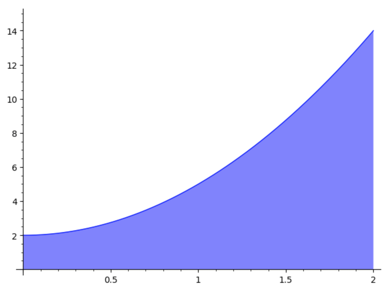
One way to do this is to use rectangles to approximate the area of \(R\). When we use the area of rectangles to approximate the area of a bounded region we compute what is called a Riemann sum.
Steps for computing Riemann sums
- Partition the interval \( [a,b]\) into \(n\) subintervals of equal width, \( \Delta x = \dfrac{b-a}n \).
- Generate \(n\) rectangles of equal widths \( \Delta x\).
- The height of each rectangle is determined by a value of the function over that subinterval. We can use the value of the function at the left endpoint of the subinterval, at the midpoint of the subinterval, at the right endpoint of the subinterval, or at a random \( x\) value in that subinterval.
- Put together, the rectangles form a polygon whose area approximates the area of \(R\).
For example, we can approximate the area of the region bounded by \( f(x) = 3x^2 + 2 \), the horizontal axis, and the lines \( x =0 \) and \( x = 2 \) with 4 rectangles. Then each rectangle would have a width of \( \Delta x = \frac{2-0}{4}= 0.5 \). Such an approximation based on the values at the left endpoints is shown below.

We can use SageMath to help us compute a left Riemann sum by adding together the area of each rectangle.
f(x)=3*x^2+2Try this by copying the two lines above into the SageMath cell below.
f(0)*(0.5)+f(0.5)*(0.5)+f(1)*(0.5)+f(1.5)*(0.5)
1. Use the SageMath cell above to evaluate the right Riemann sum for the function given by your instructor on the interval given by your instructor with 4 rectangles. Record the value of \( \Delta x \) and the approximation in your lab report.